
I know what you’re thinking. A fp32 GEMM in 2026? For Ampere??
Yes, SGEMM is rarely ever used these days in the ML space given the massive compute throughput gap between CUDA and tensor cores. For reference, an A100 PCIe’s (now almost 6 years old) peak theoretical performance for bf16 is 312 TFLOPs/sec. and 156 TFLOPs/sec. for tf32, while fp32 sits at a “measly” 19.5 TFLOPs/sec. With mixed-precision
training and quantized inference being the norm, GEMM itself is practically never done in fp32 today.
Despite all of these (good) reasons, SGEMM still acts as a great learning experience for squeezing the most performance out of GPUs (without involving tensor cores, of course). In this blogpost, I will briefly go over the structure of GEMM and iteratively work through how I optimized a kernel using NVIDIA’s CUTLASS CuTe library to match/exceed cuBLAS on certain problem shapes on SM86 using my personal RTX 3070 Mobile card.
Disclaimer: this post will be for those relatively new to kernel programming, but with a basic understanding of general GPU concepts.
a brief intro on GEMMs
Large and square-ish GEMM (general matrix-multiply) routines are embarrassingly parallel and compute-bound. GPUs being massively parallel SIMT processors, they are the ideal hardware to run such algorithms on quickly.
A Simplified Model
To see why large GEMMs are compute-bound, consider an SGEMM $C = AB$ of shape $2048 \times 2048 \times 2048$.
Simplifying the memory operations to loading $A, B$ once and storing to $C$ once from/to DRAM, this results in $(2048^2 \times 3) \times 4$ bytes of movement required. The arithmetic intensity (AI) required can be computed with $2 \times M \times N \times K$, as $K$ inner products & accumulations (using FMA) are required along both $M$ and $N$ axes and dividing by the bytes of memory moved. Thus, the AI is $\frac{2(2048^3)}{3(4)(2048^2)} \approx 341$ FLOPs/byte.
Now, mapping to hardware, we use the A100 PCIe 80 GB. as an example, which has an off-chip DRAM bandwidth of $1.94$ TFLOPs/sec. and peak fp32 performance of $19.49$ TFLOPs/sec. Theoretically, with no compute roof, DRAM could allow us a blistering $1.94 \frac{\text{TB.}}{\text{sec.}} \times 341 \frac{\text{FLOPs}}{\text{byte}} \approx 661 \frac{\text{TFLOPs}}{\text{sec.}}$. However, since the underlying fp32 ALUs are capped at $19.49$ TFLOPs/sec., we are compute-bound. Note that in reality, we will almost never reach either of these roofs, as we will later see.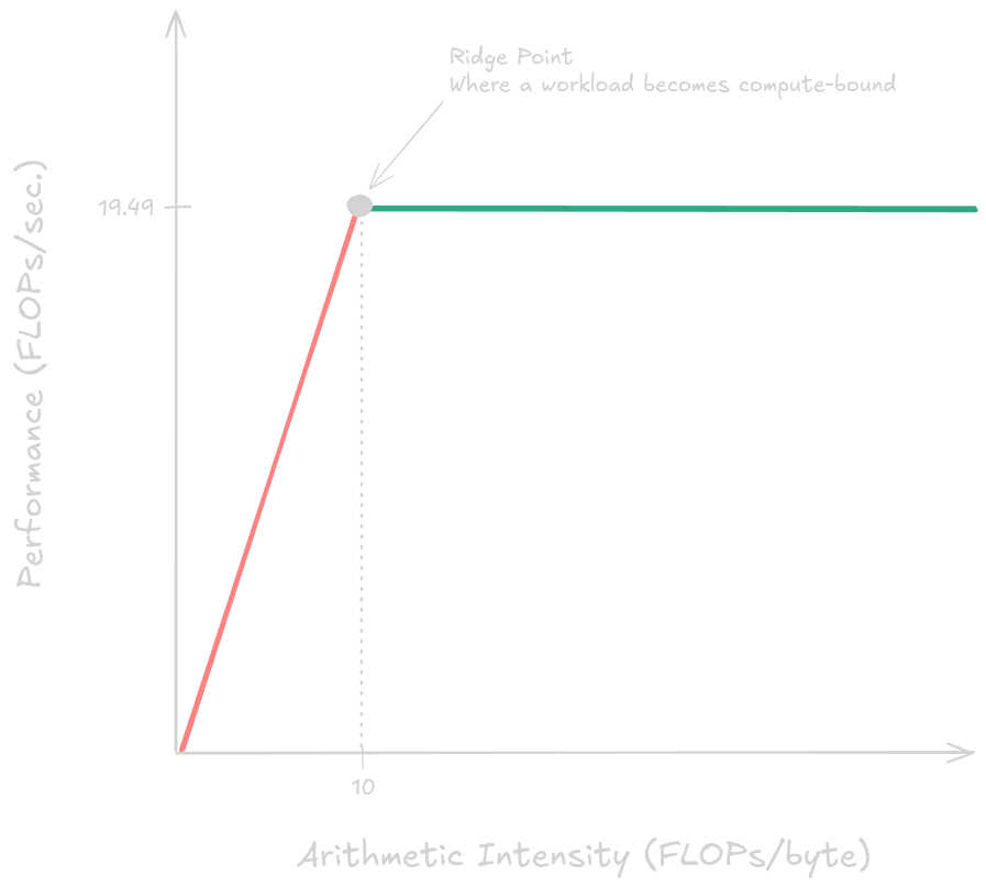
fp32 ridge point (not to scale)
For a more detailed explanation of the roofline model, see Modal’s glossary .
So the goal is straightforward: keep compute units busy by making sure data is always there when they need it. This pushes us towards using faster levels of the CUDA memory hierarchy. This includes the non-programmable L1 and L2 caches, and programmable shared memory (SMEM) and registerfile. These on-chip memory regions are much smaller in size, but have far higher throughput than DRAM. A more detailed discussion of these memory levels is available in the CUDA docs .
The basic hardware unit of NVIDIA GPUs is the streaming multiprocessor (SM), which contains shared memory, the registerfile, ALUs, LSUs, warp schedulers, and more. Warp schedulers issue instructions for warps to execute in lockstep (barring warp divergence), and can swap executing warps extremely quickly when some are in a blocked state, enabling latency hiding.
To exploit this memory hierarchy and the large data reuse inherent to GEMM, most large routines follow a similar pattern: tile and move $A, B$ into SMEM and loop along the $K$-axis for each thread/warp to accumulate its own small outer product tile within the SMEM tile. See the basic pseudocode below. With the introduction of tensor cores, the motivation for tiling became stronger, as these specialized hardware units execute warp-wide mini-GEMMs on specific tile shapes. Newer microarchitectures like Hopper (SM90) and Blackwell (SM100+) also have WGMMA, TMA, and TMEM, which are asynchronous hardware units that can accelerate such routines greatly.
// SMEM tiles
__shared__ float A_tile[block_M * block_K];
__shared__ float B_tile[block_K * block_N];

// chunking along K-axis
const int tiles = CEIL_DIV(K, block_K);

// thread-local accumulator in registerfile
float C_accum[thread_M * thread_N] = {0.0};
// outer-product operands
float A_register[thread_M] = {0.0};
float B_register[thread_N] = {0.0};

for (int tile = 0; tile < tiles; ++tile) {
    for (int load_tile = 0; load_tile < A_load_tiles; ++load_tile) {
        // ...LDGSTS A SMEM tile
    }
    for (int load_tile = 0; load_tile < B_load_tiles; ++load_tile) {
        // ...LDGSTS B SMEM tile
    }
    __syncthreads();
    for (int k = 0; k < block_K; ++k) {
        for (int m = 0; m < thread_M; ++m) {
            // ...LDS A outer product operand
        }
        for (int n = 0; n < thread_N; ++n) {
            // ...LDS B outer product operand
        }
        for (int m = 0; m < thread_M; ++m) {
            for (int n = 0; n < thread_N; ++n) {
                // ...accumulate outer products
            }
        }
    }
    __syncthreads();
}
for (int m = 0; m < thread_M; ++m) {
    for (int n = 0; n < thread_N; ++n) {
        // ...STG accumulated registerfile
    }
}

// LDG = read from DRAM, STG = write to DRAM
// LDS = read from SMEM, STS = write to SMEM
Unfortunately for us, Ampere does not have such features. The closest equivalent is the hardware-backed cp.async family of instructions, which allow a warp to asynchronously transfer memory from DRAM to SMEM (one-way), bypassing the registerfile without blocking. Note that cp.async requires every thread in a block to cooperatively load a tile into SMEM, unlike TMA. Still, this instruction will come in handy, as we can asynchronously load the next tile of data into a circular SMEM buffer while the current tile is being processed to keep compute units busy.
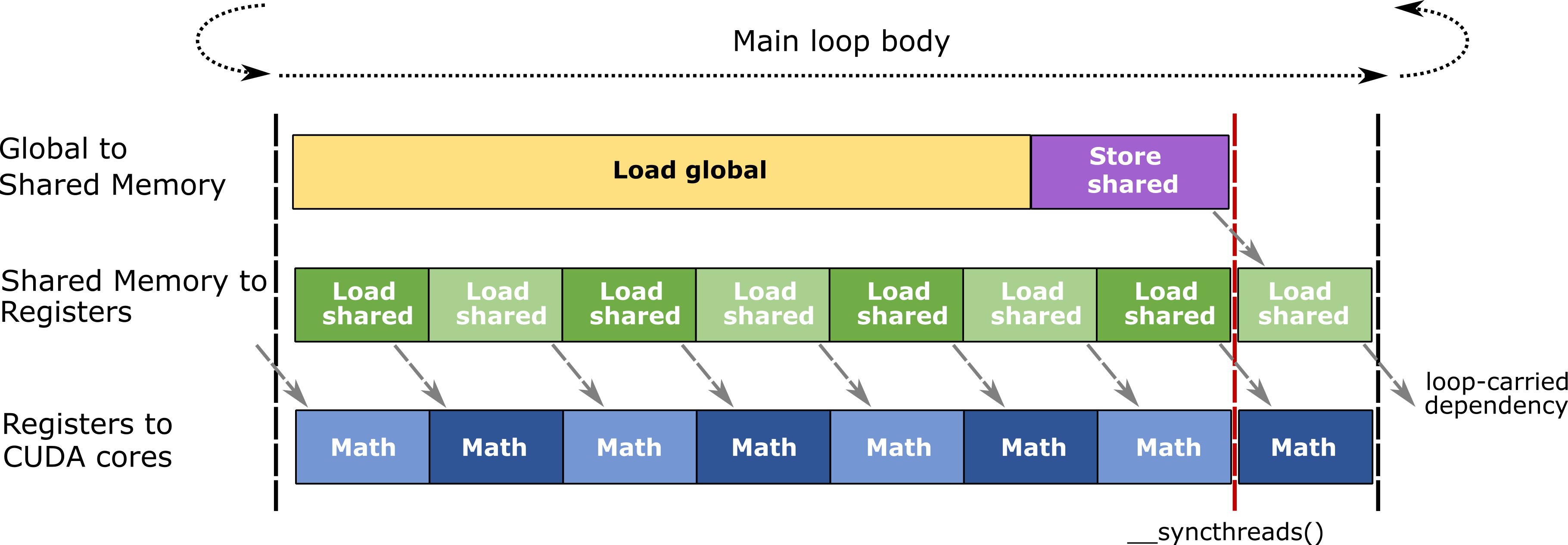
We use a similar pipelining technique when moving data to the registerfile from SMEM. We allocate 2 “$K$-slices” worth of operand data (or as we will call them — blocks) from $A, B$ and have each register-backed buffer swap between compute and reading the next blocks from SMEM (more in-depth discussion later). This diagram from NVIDIA outlines the approach well:
host-side setup
With all that being said, let’s setup the kernel! We’ll hand off most of the indexing calculations to CuTe to deal with at compile-time, so that we can save some of our precious registers. We’ll start with the necessary setup on host-side. This will be a nn kernel, where both inputs are not transposed and expected to be in column-major format.
void nn(int m, int n, int k,
        float alpha, const float* A, int ldA,
        const float* B, int ldB, float beta,
        float* C, int ldC, cudaStream_t stream = 0) {
    using namespace cute;

    auto cta_shape = make_shape(Int<128>{}, Int<128>{}, Int<32>{});
    auto stride_A = make_stride(Int<1>{}, ldA);
    auto stride_B = make_stride(ldB, Int<1>{});
    auto stride_C = make_stride(Int<1>{}, ldC);

    constexpr int n_pipes = 3;
    auto sA_layout = make_layout(make_shape(select<0>(cta_shape), select<2>(cta_shape), Int<n_pipes>{}));
    auto sB_layout = make_layout(
        make_shape(size<1>(cta_shape), size<2>(cta_shape), Int<n_pipes>{}),
        make_stride(size<2>(cta_shape), Int<1>{}, size<1>(cta_shape) * size<2>(cta_shape))
    );
    constexpr uint smem_size = (cosize_v<decltype(sA_layout)> + cosize_v<decltype(sB_layout)>) * sizeof(float);
    ...
}We define the SMEM tiling shapes for $A, B$ to be $128 \times 32$, and the strides for their entire tensors in DRAM to be column-major. The DRAM and SMEM $B$ tile shapes are $(N, K)$ rather than the usual $(K, N)$ to consistently keep the reduction mode $K$ on the right, like $A$, which is $(M, K)$. For the SMEM tiles, we’ll use a 3-stage circular buffer for both. To use the widest granularity for reads/writes (i.e. 128-bits), both SMEM tiles should also be in column-major. Wider reads and writes lower instruction count and generally improve performance.
cp.asynccan move memory at 4-, 8-, and 16-byte granularities. Furthermore, reads from DRAM AND writes to SMEM must strictly be to contiguous chunks of memory.
CuTe Layouts
A CuTe tensor is comprised of an iterator and Layout, which is a potentially nested tuple of a Shape and Stride, which themselves are potentially nested tuples. The layout is convenient because it informs us of the logical shape of a tensor and the “contiguity” of the elements, which is very important when writing kernels. However, at its core, a layout is simply a function from $Z^n \rightarrow Z$ that results in a linear offset by computing a dot product between an input $n$-mode tuple (coord) and the layout’s stride. Lastly, CuTe uses colexiographical order; it always “fills” a layout starting from the left-most mode moving to the right.
There are many great resources out there that helped me formally understand the layout concept, like Colfax Research’s paper and Lei Mao’s blogpost . The two can be pretty dense with the math though, so the good old documentation from the CUTLASS team helped me out here a lot too.
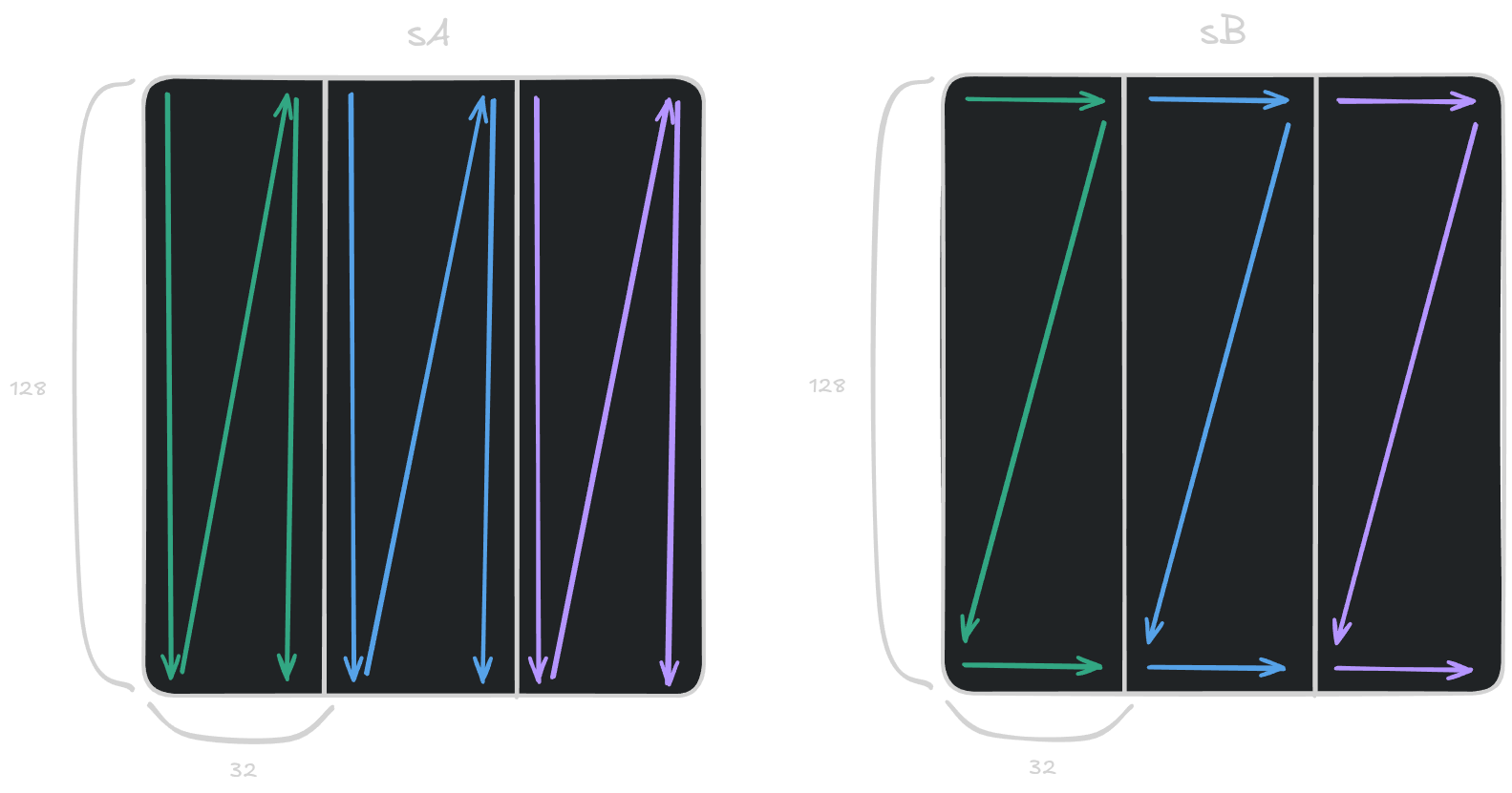
sA_layout and sB_layout.
We sum up the cosizes of each SMEM layout to retrieve the number of bytes of SMEM required for the kernel. We need to dynamically allocate SMEM in our kernel, as CUDA caps static allocation at 48 kilobytes across all microarchitectures (we need $128 \times 32 \times 3 \times 2 \times 4 = 98304$ bytes).
A side note: Cosize represents the size of the codomain of a layout. When a layout is compact and bijective, the size is equivalent to the cosize. However, there may be times where this is not the case:
- It has “gaps” in the codomain (i.e. non-compact but bijective), in which its cosize will be greater than its size.
- Non-injective layouts, when multiple coordinates in the domain map to the same value in the codomain (e.g. broadcasting), where its cosize is less than its size.
For us, the SMEM layouts are compact and bijective. We still use cosize though to enforce that they require the minimum size of the codomains to back their layouts in physical memory, independent of the tensors’ logical size.
auto copy_A = make_tiled_copy(
    Copy_Atom<Copy_Traits<SM80_CP_ASYNC_CACHEGLOBAL<uint128_t>>, float>{},
    make_layout(make_shape(Int<32>{}, Int<8>{})),
    make_layout(make_shape(Int<4>{}, Int<1>{}))
);
auto copy_B = make_tiled_copy(
    Copy_Atom<Copy_Traits<SM80_CP_ASYNC_CACHEGLOBAL<uint128_t>>, float>{},
    make_layout(make_shape(Int<32>{}, Int<8>{}), LayoutRight{}),
    make_layout(make_shape(Int<1>{}, Int<4>{}), LayoutRight{})
);
auto mma = make_tiled_mma(
    MMA_Atom<UniversalFMA<float>>{},
    Layout<Shape<_16,_16>>{}
);
auto kernel = ampere_sgemm_128x32_3stage<decltype(stride_A), decltype(stride_B), decltype(stride_C),
                                         decltype(sA_layout), decltype(sB_layout), decltype(cta_shape),
                                         decltype(copy_A), decltype(copy_B), decltype(mma)>;
cudaFuncSetAttribute(kernel, cudaFuncAttributeMaxDynamicSharedMemorySize, smem_size);
cudaFuncSetAttribute(kernel, cudaFuncAttributePreferredSharedMemoryCarveout, 100);

dim3 block_dim(size(mma));
dim3 grid_dim(size(ceil_div(m, select<0>(cta_shape))), size(ceil_div(n, select<1>(cta_shape))));
kernel<<<grid_dim, block_dim, smem_size, nullptr>>>(
    m, n, k, alpha, beta, A, stride_A, B, stride_B, C, stride_C, cta_shape, sA_layout, sB_layout, copy_A, copy_B, mma
);Setting up the tiled MMA and copy objects, there’s a bit of boilerplate code needed.
make_tiled_copy allows us to arrange a group of threads with a certain layout and assign a group of elements for each thread to be responsible for. We wrap a CopyTraits object to use the SM80 cp.async.cg.shared.global.L2::128B instruction with a read granularity of 128-bits = 16-bytes. The CopyAtom then takes this CopyTraits and the actual dtype to be used.
The layout of the threads for $A$ is $(32 \times 8)$ in column-major, with each thread responsible for 4 column-major elements, whereas for $B$ both are in row-major arrangement. It is very important to write correct layouts for any problem to ensure read-write access patterns that we actually intended (CuTe will also statically fail if given an impossible access pattern).
A good way to start writing these is to write out the ideal case, or what we’d expect the tiling to be. To coalesce 128-byte DRAM reads and use thread-local 16-byte loads, there should be a stride of 1 between each thread’s 4 fp32s and stride of 4 between threads.
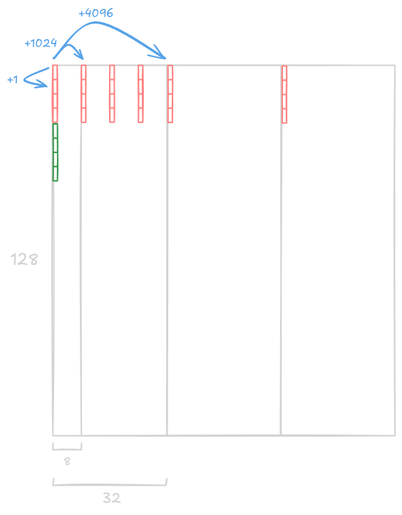
Above is an ideal partitioning of the destination tensor. We can see some values mapped to Thread 0 in pink. The green represents the first 4 values mapped to Thread 1. Thread 2’s values would be right below, and so on, tiling in column-major order. The blue represents the actual stride required in physical linear memory to jump to the next value. The stride-1 between each value within the 4-value blocks allow us to use the wide 16-byte instructions. This layout also maximally coalesces GMEM (global memory) transactions.
Coalescing & Global Memory
Recall that any GMEM read fetches a contiguous 128-byte cache line into L2 at minimum. When every thread in a warp reads a contiguous, adjacent element, the hardware coalesces those 32 requests into the minimum number of cache lines. With our layout, 32 threads × 16 bytes = 512 bytes = 4 cache lines. In the worst case, with strided accesses, each thread could require its own cache line fetch, multiplying transaction count by up to 32. Note that coalescing applies to accesses of threads within a warp, not across warps.
Just to verify, we can print copy_A.tidfrg_D(dst_tensor):
$$ (256,(4,1),(1,4,3)):(4,(1,0),(0,1024,4096)) $$
The comments in CuTe source code for tidfrg_S and tidfrg_D explain what these layouts represent:
// Tile a tensor or a layout from shape
//   (M,N,...)
// to shape
//   (Thr,(FrgV,FrgX),(RestM,RestN,...))
// where
//   Thr:   The logical threads within the tiled copy.
//   FrgV:  The values local to a COPY_ATOM Dst.
//   FrgX:  The values tiled across COPY_ATOMs Dst.
//   RestM: The values tiled in M.
//   RestN: The values tiled in N.
auto tidfrg_D(DTensor&& dtensor) {
    ...
}Corresponding each term to what we saw, we see that this tiled copy uses 256 threads, where each thread is mapped to 4 values local to a copy atom (16-byte cp.async atom = 4× fp32), 4 values tiled across the K-mode, and 3 values tiled across the shared memory’s 3 stages, matching our earlier visualization. Internally, partition_X uses the layouts from tidfrg by indexing the Thr-mode with the thread index in the actual kernel.
Occupancy & Parallelism
You may be asking how we chose the number of threads to use. GPUs have constrained on-chip memory sizes. For compute-bound problems, we typically prefer loading larger tile sizes to faster on-chip memory since data reuse is high. Fetching data from HBM once for larger tiles and reusing it from shared memory or registers helps amortize that memory latency across more arithmetic operations.
However, this comes at a price — heavier on-chip memory usage reduces occupancy, the number of warps (group of 32 threads) resident on an SM. Fewer warps means the scheduler may not be able to switch to another warp when one is “blocked”, potentially preventing latency hiding. This occupancy vs. arithmetic intensity tradeoff is an important concept that informs us of a kernel’s optimal launch configuration.
Lastly, we set up a TiledMMA object, which assigns threads to values for matrix-multiply accumulation (MMA). Similar to TiledCopy, it takes an MMA_Trait wrapping an MMA_Atom, which defines the smallest “unit” of computation to be tiled. This allows for easy partitioning of the operand $A$ and $B$ matrices and register allocation for the product $C$ fragment. Since our operands are in fp32, which don’t have tensor core support, we use the UniversalFMA<float> atom here. But, for example, if our operands were to be in half-precision, we’d want to use an atom like SM80_16x8x16_F16F16F16F16_TN that wraps a tensor core (TC) instruction.
Each of these atoms intrinsically involve a different number of threads. For FMA, it’s just 1 thread performing a scalar computation. Ampere TC instructions are at warp-level; they require a warp to cooperatively compute a small matrix product, while Hopper TCs involve a warpgroup (4 warps) and so on. We’ll focus on the simple FMA case.
Suppose that after we’ve done some tuning, we decide to use 256 threads in our kernel. Of course, writing a kernel for first time, you wouldn’t know the optimal number of threads, but 128 or 256 threads tend to be good starting points for GEMMs. With each thread computing 1 scalar fragment of $C$, a threadblock of 256 threads can independently compute 256 $C$ values per atom. For balanced data reuse, we’ll arrange the atom’s 256 values to compute a $(16 \times 16)$ fragment of $C$.
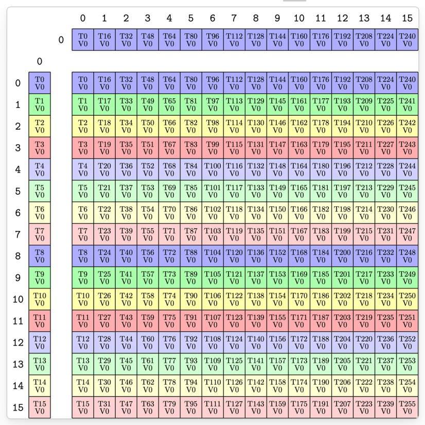
print_latex helps us visualize the atom. Each thread computes 1 scalar product and accumulates to its 1 fragment register.
You may be asking: “But I thought our setup was for each threadblock to accumulate a $(128 \times 128)$ tile of $C$?” TiledMMA exposes similar methods to TiledCopy, where we can partition an arbitrarily-sized input tensor according to this smaller atom layout. In other words, it replicates the atom across given matrices. Partitioning a $(128 \times 128)$ tile of $C$ thus results in an $(8 \times 8)$ tile of atoms. There is also thrfrg, which is the MMA equivalent to the tidfrg from TiledCopy we saw earlier. Printing thrfrg_C(gC).shape:
$$ ((1, (16, 16)), (1, (8, 8))) $$
And again, looking at the source code comments:
// Tile a tensor or a layout from shape
//   (M,N,...)
// to shape
//   ((ThrV,(ThrM,ThrN)),(FrgV,(RestM,RestN,...)))
// where
//   ThrV:  The threads local to an MMA. layout<0>(ThrLayoutVMNK): ThrV -> thread_idx
//   ThrM:  The threads tiled in M.      layout<1>(ThrLayoutVMNK): ThrM -> thread_idx
//   ThrN:  The threads tiled in N.      layout<2>(ThrLayoutVMNK): ThrN -> thread_idx
//   FrgV:  The values local to an MMA.
//   RestM: The values tiled in M.
//   RestN: The values tiled in N.
auto thrfrg_C(CTensor&& ctensor) const {
    ...
}We see that there is exactly 1 thread and 1 value local to the MMA atom, and 16 threads tiled in the M- and N-modes. To cover the entire threadblock tile, there then must be 8 values tiled in the M- and N-modes too, meaning the $C$ fragment alone requires 64× 32-bit registers per thread. That is, each thread is computing an $(8 \times 8)$ outer product. Let’s look at thrfrg_A now:
$$((1,(16,1)),(1,(8,32,3)))$$
Notice here how no threads are tiled in the K-mode. Instead, each thread owns all values in its K-mode, as it requires an accumulation over this mode. Now, we can move onto the block/thread-local setup within the actual kernel.
device-side setup
// cta_shape is (Tile M, Tile N, Tile K) = (128, 128, 32)
auto mA = make_tensor(make_gmem_ptr(A), make_layout(make_shape(m, k), stride_A));
auto mB = make_tensor(make_gmem_ptr(B), make_layout(make_shape(n, k), stride_B));
auto mC = make_tensor(make_gmem_ptr(C), make_layout(make_shape(m, n), stride_C));

auto coord = make_coord(blockIdx.y, blockIdx.x, _);
auto gA = local_tile(mA, cta_shape, coord, Step<_1, X, _1>{});
auto gB = local_tile(mB, cta_shape, coord, Step<X, _1, _1>{});
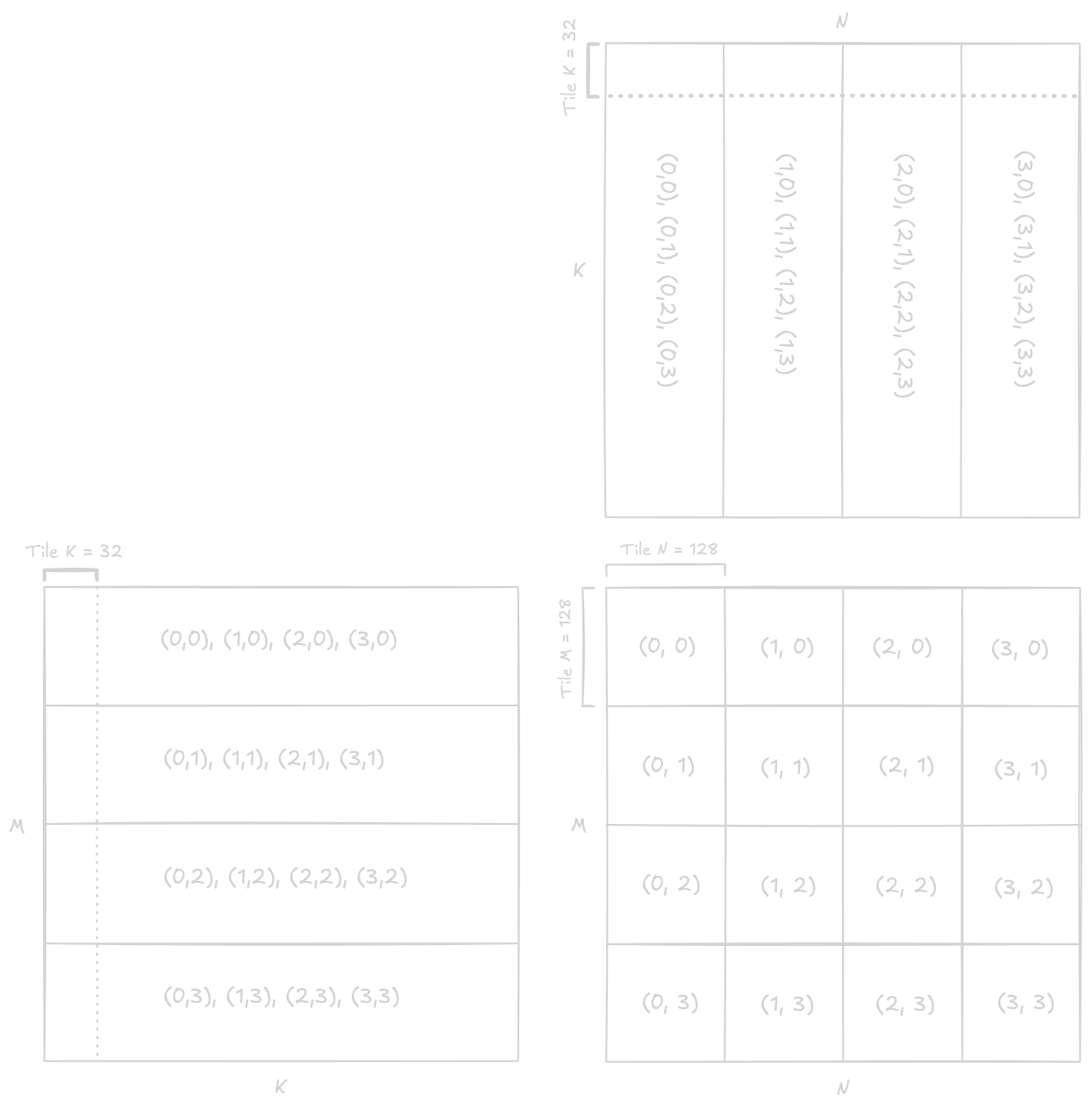
auto gC = local_tile(mC, cta_shape, coord, Step<_1, _1, X>{});This code is boilerplate for GEMMs. We first create the dynamically-shaped global memory tensors. To “assign” each $(M, N)$ tile coord to threadblocks, we create a Coord object based on block index, and use the local_tile API. Internally, this function is a wrapper on top of zipped_divide that take Coord and Step objects, which specify which tile coord we want to slice out and which modes we want to keep/discard, respectively. Notice the X in the Step object, which means that the corresponding mode in the cta_shape divisor is dropped. Since it’s of shape $(\text{Tile M, Tile N, Tile K})$, we specify the X at mode-1 for $A$ and mode-0 for $B$.
For example, for gA, this means we index mode-0 of the “quotient” tensor of shape $\left(\frac{M}{\text{Tile M}}, \frac{K}{\text{Tile K}}\right)$ by blockIdx.y and keep all of mode-1, since each block does a reduction along the K-mode. Thus, we set Coord to (blockIdx.y, blockIdx.x, _) — in CuTe syntax, an underscore indicates we keep all of that mode. This results in gA and gB of shape $(128, K)$.
extern __shared__ float smem_buffer[];
auto sA = make_tensor(make_smem_ptr(&smem_buffer[0]), sA_layout);
auto sB = make_tensor(make_smem_ptr(&smem_buffer[cosize_v<sALayout>]), sB_layout);

auto tA = copy_A.get_thread_slice(threadIdx.x);
auto tAgA = tA.partition_S(gA);
auto tAsA = tA.partition_D(sA);

auto tB = copy_B.get_thread_slice(threadIdx.x);
auto tBgB = tB.partition_S(gB);
auto tBsB = tB.partition_D(sB);We then setup the shared memory tensors from a single buffer, and partition the source and destination tensors for each thread based on the TiledCopy objects we discussed earlier. Printing tAsA.shape from any thread gives us $(4, 1), 1, 4, 3$. We can see that this is exactly what we saw from tidfrg_D, but without mode-0, since we’ve now sliced that tensor to get the thread-local partition. Similarly, tAgA.shape prints $(4, 1), 1, 4, 32$ when $K = 1024$, as $\frac{1024}{\text{Tile K}} = 32$ (mode-3 represents values tiled across $K$).
using blockPipes = _2;  // num. of block buffers
...
auto tC = tiled_mma.get_thread_slice(threadIdx.x);
auto tCsA = tC.partition_A(sA);
auto tCsB = tC.partition_B(sB);
auto tCgC = tC.partition_C(gC);
auto tCrA = make_fragment_like(composition(tCsA(_,_,_,0), make_shape(_,_,blockPipes{})));
auto tCrB = make_fragment_like(composition(tCsB(_,_,_,0), make_shape(_,_,blockPipes{})));
auto tCrC = make_fragment_like(tCgC);
fill(tCrC, 0.0);Last component for the setup is now setting up the thread-local MMA registers. TiledMMA already gave us a thread-value mapping for $A$, $B$, and $C$, so we just need to slice out each thread-local view and partition the input tensors. Notice that gC is referring to the global memory pointer for $C$, since we’re not tiling it into SMEM, only $A$ and $B$.
You may be asking what this is doing: composition(tCsA(_,_,_,0), make_shape(_,_,blockPipes{})). Recall the pipelining diagram from before, and how each thread owns all of its K-mode. Ideally, we want each thread to begin its load for the next “slice” of its K-mode from SMEM while doing compute on this current slice to save some cycles. The cost though is that we require more registers to eliminate the potential scoreboard stall, hence why we set blockPipes to 2.
Scoreboard
In CUDA, the scoreboard is a memory dependency tracking system. It dynamically ensures that instructions that depend on some overlapping memory run in an order that preserves correctness (more on this from Modal ). Consider this pseudocode:
// single register
float a_reg, b_reg;
for (k = 0 ... Tile K) {
    a_reg = sA[k];  // LDS
    b_reg = sB[k];  // LDS
    c += a_reg * b_reg;  // FMA (stalls until LDS completes)
}Because the FMA on any iteration reads from the same registers that the LDS on that iteration writes to, a scoreboard dependency is created — the FMA stalls until both loads complete, despite the fact that they could run on independent hardware units on an SM (LDS on load/store units, FMA on CUDA cores). Visualizing this for one of the operands…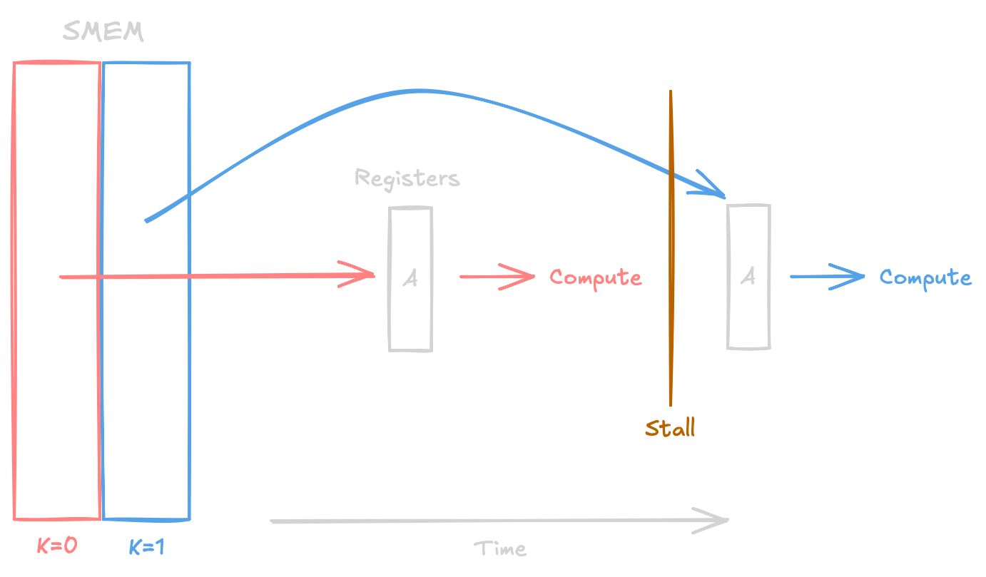
LDS for $K = 1$ before or during FMA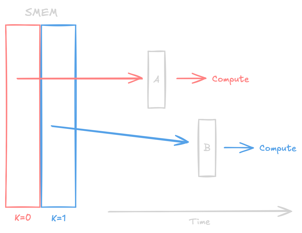
LDS for the next tile with the FMA for the current tile.
Note we are at the mercy of the compiler here. It’s up to us as the programmer to semantically express the dependency-free condition as clearly as possible and verify that the compiler has generated the correct SASS (nsight-compute is good for this). However, ptxas tends to be good at optimizing these kinds of common pipeline routines.
If you have some experience in performance optimization, you’re probably familiar with this kind of software pipelining. What this typically looks like is scheduling a high latency instruction prior to executing another independent instruction, so that the former does not hurt throughput and they can run on different hardware units. This enables ILP (instruction-level parallelism) — attempting to exploit parallelism on an instruction-scheduling basis within each warp’s instruction stream.
Note that this is not the only way to expose ILP. Another common technique is unrolling a loop if it’s bound by a compile-time constant. Since compute/load/store instructions are pipelined and have an associated latency, we can schedule multiple independent instructions of the same type to saturate a hardware unit. This way, for example, one FMA may be on cycle 2/4 while another independent one may be on cycle 1/4 on the same ALU.
Recall from our TiledMMA discussion earlier that thrfrg_A mapped 8 values in the M-mode and all 32 values in the K-mode to each thread. The motivation of the composition(...) is to only have blockPipes values in the K-mode physically allocated in registers, since allocating the entire K-mode may cause register spilling (8 × 32 = 256 registers for 1 operand alone!). Recall register spilling occurs when each thread requires over a certain number of registers (depends on occupancy) and causes the compiler to store registers in local memory (physically backed by slow DRAM) instead, hurting performance.
tCsA(_,_,_,0) globs all the values local to the MMA Atom (1), values tiled in the M-mode (8), and tiled in the K-mode (32). The 0 in the last mode specifies that we just want the values local to one SMEM pipe. We then compose (roughly analagous to functional composition) this sub-tensor with a shape that is identity for values local to the MMA Atom and tiled in the M-mode, but restricts the K-mode values to blockPipes.
mainloop
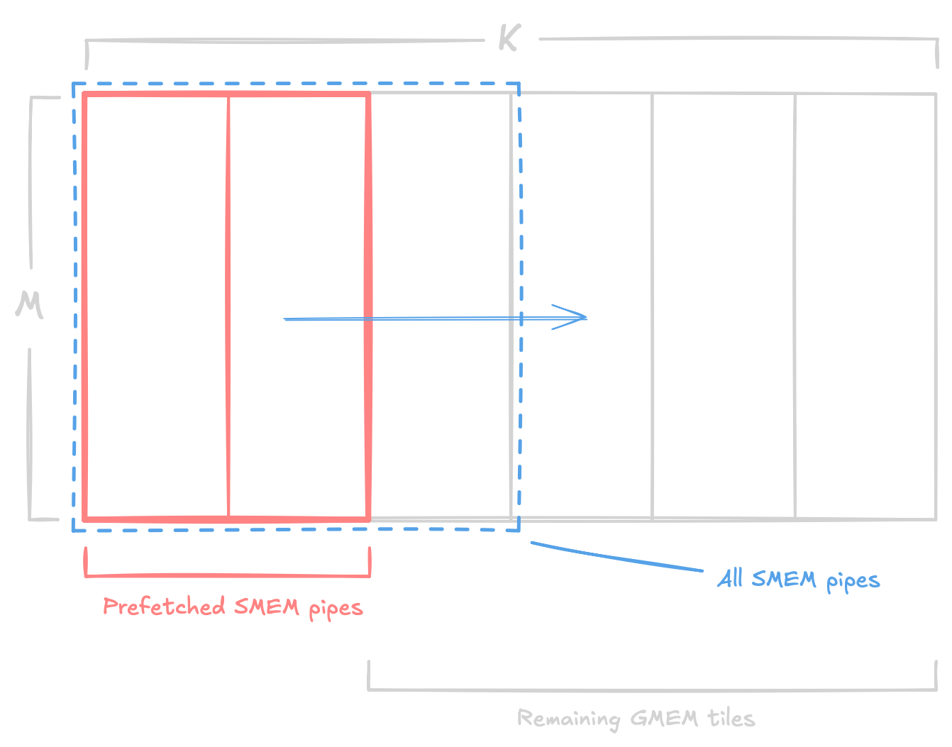
We’ll now implement the mainloop, where each threadblock loops over its K-tiles and accumulates its individual matrix product. We begin with a prefetch to avoid some extra conditional statements inside the loop.
uint gmem_tile_idx = 0;
uint gmem_tiles = size<2>(gA);
constexpr uint smem_pipes = size<2>(sA);

// prefetch for first (smem_pipes - 1) pipes
CUTE_UNROLL
for (uint i = 0; i < smem_pipes - 1; ++i) {
    copy(copy_A, tAgA(_,_,_,gmem_tile_idx), tAsA(_,_,_,i));
    copy(copy_B, tBgB(_,_,_,gmem_tile_idx), tBsB(_,_,_,i));
    cp_async_fence();
    --gmem_tiles;
    if (gmem_tiles) {
        ++gmem_tile_idx;
    }
}We initialize some variables for tracking:
gmem_tile_idxto track which global K-tile is next to be loadedgmem_tilesis the number of total K-tiles, equal to $\frac{K}{\text{Tile K}}$ (cannot beconstexprif $K$ is a runtime value)smem_pipesis the number of shared memory pipes (in our case — 3)
In the prefetch loop, we fire off the loads for the first 2 out of 3 pipes. For each copy call, we glob the values local to a copy atom, values tiled across Tile M, and values tiled across Tile K by placing an underscore at those modes. We then copy this K-tile at position gmem_tile_idx to the corresponding pipe. Lastly, we decrement the number of K-tiles left to load, and only increment the K-tile position if there are more left. Otherwise, the next iteration simply loads the same global K-tile into the next pipe to prevent a segfault.
Async Copy
To use cp.async effectively, CuTe provides two key functions:
cp_async_fence()wraps thecp.async.commit_groupPTX instruction, which “commits all prior initiated but uncommittedcp.asyncinstructions into a cp.async-group.” (NVIDIA)- This is effectively a code barrier that allows us to create logical groups of loads, so that we can wait for certain groups to finish before doing some work, while intentionally allowing others to continue.
cp_async_wait<N>()wraps thecp.async.wait_groupinstruction, which “will cause executing thread to wait till only N or fewer of the most recent cp.async-groups are pending and all the prior cp.async-groups committed by the executing threads are complete.” (NVIDIA)- This gives us the aforementioned ability to wait for certain groups to finish. The fences create an implicit queue, and this instruction lets us “pop off” a specified number of pending groups from the front of the queue.
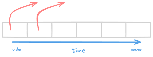
An example of 6 committed groups and a cp_async_waitcall with N=4. Guarantees that at most 4 groups are pending (may be less) and anything older is completed.
- This gives us the aforementioned ability to wait for certain groups to finish. The fences create an implicit queue, and this instruction lets us “pop off” a specified number of pending groups from the front of the queue.
Given our discussion earlier on ILP and overlapping certain instructions, you may be wondering why cp.async was such a powerful introduction with Ampere chips. Why can’t we just run a standard LDG (load from global memory) instruction while doing compute on the current tile? The 2 biggest benefits from using cp.async instead are:
- Global memory loads do not take up registers. Standard
LDGstages memory through registers first before reaching SMEM, consuming valuable registers and leaving less for compute-intensiveFMA/MMAinstructions. - We have fine-grained control over memory visibility and synchronization.
- For GEMM, the values mapped to each warp for GMEM to SMEM loads are often different from the values mapped for SMEM to registerfile loads. Since warps depend on other warps to load data before their inner accumulation loops, we need to ensure shared memory visibility to the entire threadblock. We use the
__syncthreadsruntime barrier, waiting until all warps arrive, in between GMEM to SMEM loads and SMEM to register loads. - Using standard
LDGinstructions instead forces all GMEM to SMEM loads to complete, including those for succeeding tiles we don’t need at the moment, because we don’t have the fine-grained control to selectively wait on certain loads. cp.asyncdecouples the threadblock-wide execution barrier from the loads, allowing us to use__syncthreadsto ensure SMEM visibility, while still giving us flexibility on the synchronization of the loads. We’ll see this in action later in the mainloop.
- For GEMM, the values mapped to each warp for GMEM to SMEM loads are often different from the values mapped for SMEM to registerfile loads. Since warps depend on other warps to load data before their inner accumulation loops, we need to ensure shared memory visibility to the entire threadblock. We use the
And for the last setup bits before the actual loop body, we do a prefetch for the first register block from SMEM. Note that we need to wait until just the first tile is loaded using cp_async_wait<1> and sync the threadblock for visibility.
int block_pipe = 0;
cp_async_wait<smem_pipes - 2>();
__syncthreads();
// prefetch rmem_block = 0
copy(tCsA(_,_,0,0), tCrA(_,_,block_pipe));  // (M, K, pipe)
copy(tCsB(_,_,0,0), tCrB(_,_,block_pipe));  // (N, K, pipe)

uint pipe_read = 0;
uint pipe_write = smem_pipes - 1;
constexpr uint rmem_blocks = size<2>(tCsA);
const uint k_iters = gmem_tiles + (smem_pipes - 1);Finally, we set some variables for tracking the pipeline stages. pipe_read and pipe_write correspond to the SMEM pipe to read from and write to, respectively. rmem_blocks is the number of values tiled across the K-mode of the SMEM tile (32) and k_iters tracks the number of GMEM tiles left after the prefetch and to drain the prefetched SMEM pipes.
for (uint iter = 0;  iter < k_iters; ++iter) {
    if (iter < gmem_tiles) {
        copy(copy_A, tAgA(_,_,_,gmem_tile_idx), tAsA(_,_,_,pipe_write));
        copy(copy_B, tBgB(_,_,_,gmem_tile_idx), tBsB(_,_,_,pipe_write));
    }
    cp_async_fence();

    CUTE_UNROLL
    for (uint block = 0; block < rmem_blocks - 1; ++block) {
        copy(tCsA(_,_,block+1,pipe_read), tCrA(_,_,block_pipe^1));  // TODO: call before gemm to interleave?
        gemm(tiled_mma, tCrA(_,_,block_pipe), tCrB(_,_,block_pipe), tCrC);
        copy(tCsB(_,_,block+1,pipe_read), tCrB(_,_,block_pipe^1));
        block_pipe ^= 1;
    }
    gemm(tiled_mma, tCrA(_,_,block_pipe), tCrB(_,_,block_pipe), tCrC);
    block_pipe ^= 1;
...We begin the loop body by checking if there’s another K-tile still left to process. If so, we fire off the async copy for that GMEM → SMEM load, and group it with the fence, which will go into our last (3rd) SMEM pipe. Note that the fence is placed outside the if-statement, which creates empty copy groups for tail iterations where there are no new GMEM tiles left. This way, we ensure these tail iterations still correctly wait on their loads.
Why empty groups?
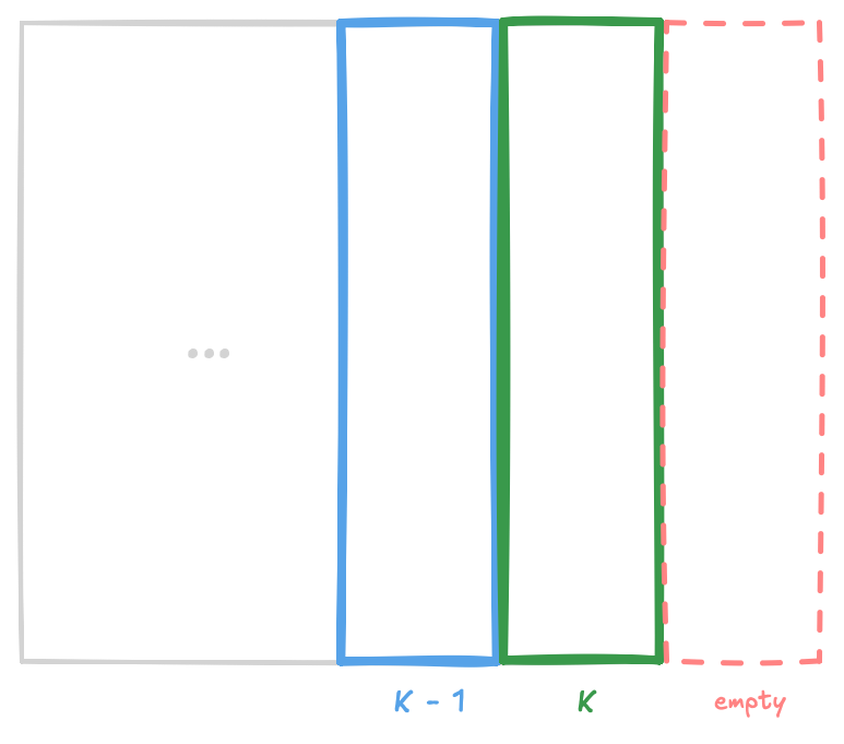
cp_async_wait<1>. The 1 here ensures that we only wait on the $K^{\text{th}}$ tile, and not the $(K + 1)^{\text{th}}$ tile.
However, this does not exist; there is no GMEM tile left for us to preload. We thus create an empty copy group to act as a dummy position in the queue (waits on everything before) to ensure the proper wait on the last tile. Empty copy groups are trivially completable; waiting on them adds no overhead.
Some more notable things here:
copy(tCs*(_,_,block+1,pipe_read), tCr*(_,_,block_pipe^1))- For every SMEM → register copy, we move all values local to the MMA Atom and tiled across the M-mode. For the K-mode, we copy the next slice (
block + 1) from SMEM to the block pipe we’re not using in this iteration (block_pipe ^ 1). XOR lets us succintly switch between the register block used. - We specify the copy comes from the
pipe_readSMEM pipe-mode, as this is the ready-to-read sector. - We interleave the GEMM for the current tile with this copy for the next tiles of $A$ and $B$ to maximally express the potential for ILP.
- We don’t specify a
TiledCopyobject (like we did for GMEM → SMEM loads), as simple 32-bit reads are enough here.
- For every SMEM → register copy, we move all values local to the MMA Atom and tiled across the M-mode. For the K-mode, we copy the next slice (
- The
gemm(...)API automatically dispatches to an outer product calculation based on the shape of the provided operands. We also supply thetiled_mmaobject as the first arg. - We set the loop bound to run just until the last tile is left to avoid an if-statement that checks if the next block pre-load should be done, and just explicitly call the last GEMM outside of the loop.
- After each iteration, we swap and set
block_pipe, as the next iter. should use the block we pre-loaded to.
    ...
    pipe_write = pipe_read;
    pipe_read = (pipe_read + 1) % smem_pipes;

    cp_async_wait<smem_pipes - 2>();
    __syncthreads();

    if (iter != k_iters - 1) {
        copy(tCsA(_,_,0,pipe_read), tCrA(_,_,block_pipe));
        copy(tCsB(_,_,0,pipe_read), tCrB(_,_,block_pipe));
    }
    ++gmem_tile_idx;
}We then swap SMEM pipes in a “circular” fashion. Since we have processed the tile in the read pipe, we can safely overwrite it by setting it as the write pipe. The read pipe should then be set to the next tile. We modulo the incremented read pipe by the number of pipes (3) to “rotate” it back to the first pipe when it exceeds the max pipe index.
After waiting on the arrival of solely the next tile and ensuring visibility, we preload the first register fragment of the next iteration from SMEM (as long as this is not the last tile). Finally, we update the GMEM tile index for the next iteration.
epilogue
We’ll keep the epilogue pretty simple here with the standard axpby epilogue of formal GEMM implementations in BLAS libraries. Mathematically…
$$C_{\text{out}} = \alpha(AB) + \beta(C_{\text{in}})$$
…where $\alpha, \beta$ are scalars. Note that swapping in different epilogues is relatively simple. We can do this in one line of code with CuTe’s axpby API
:
axpby(alpha, tCrC, beta, tCgC);The function reads in each value of tCgC, scales it by beta, adds it to the corresponding value of tCrC scaled by alpha, and writes it back to tCgC. You may be rightly questioning the performance of this, considering every value of each thread’s 8 × 8 fragment is strided, causing narrow 32-bit reads and writes. We’ll explore the optimization for this and other issues right below.
optimizations
After verifying the kernel’s correctness, the next step is to profile and optimize performance. NVIDIA’s nsight-compute application provides key metrics and suggestions by profiling kernels, helping us quickly narrow down on bottlenecks. We can launch it via terminal:
ncu --set full --open-in-ui ./my_kernel <args...>swizzles & shared memory
Upon profiling, ncu informs us of a problem about our use of shared memory:
Shared Memory Banks
Shared memory on NVIDIA GPUs is organized into 32 banks, each 4 bytes wide. Each of these banks can service exactly one 4-byte word per “cycle” for a warp. The term cycle here is defined loosely; we’re talking about the smallest possible unit of time that a bank can fulfill a single request.
On the software side, data is contiguously arranged into the banks from bank 0 to 31, and wrapping back around when more than 32 × 4 bytes are used. A bank conflict then occurs when lanes in the same warp attempt to access different data from the same bank. Note that if lanes try to access the same data from the same bank, this does not cause a conflict; the bank multicasts this value across the warp.
The number of banks is not just coincidentally the same as the number of threads in a warp. This was designed such that if every lane in a warp requests contiguous 4-byte (or smaller) words, the banks can fulfill the warp’s memory request in one cycle.
To illustrate, suppose we have 32 × 32 = 1024 fp32 values in shared memory as the array arr. Then, the value arr[i] at index i will be held by bank i % 32. Suppose now that thread 0 tries to read/write to arr[0], thread 1 to arr[32], and so on, until thread 31 reads/writes to arr[31 * 32]. This access pattern requires bank 0 to serialize all 32 lanes’ requests, causing a worst-case 32-way bank conflict.
In our case, an access pattern for either $A$ or $B$ in SMEM is sub-optimal. Analyzing both read/write patterns for $A$ and $B$ will be too verbose, so I’ll tell you right now that the read pattern for $B$ is the issue, leaving the other patterns for you as exercises.
Recall from our tiled MMA layout that each group of 16 consecutive threads share the same “N-row”. Visualizing the $B$ read pattern:
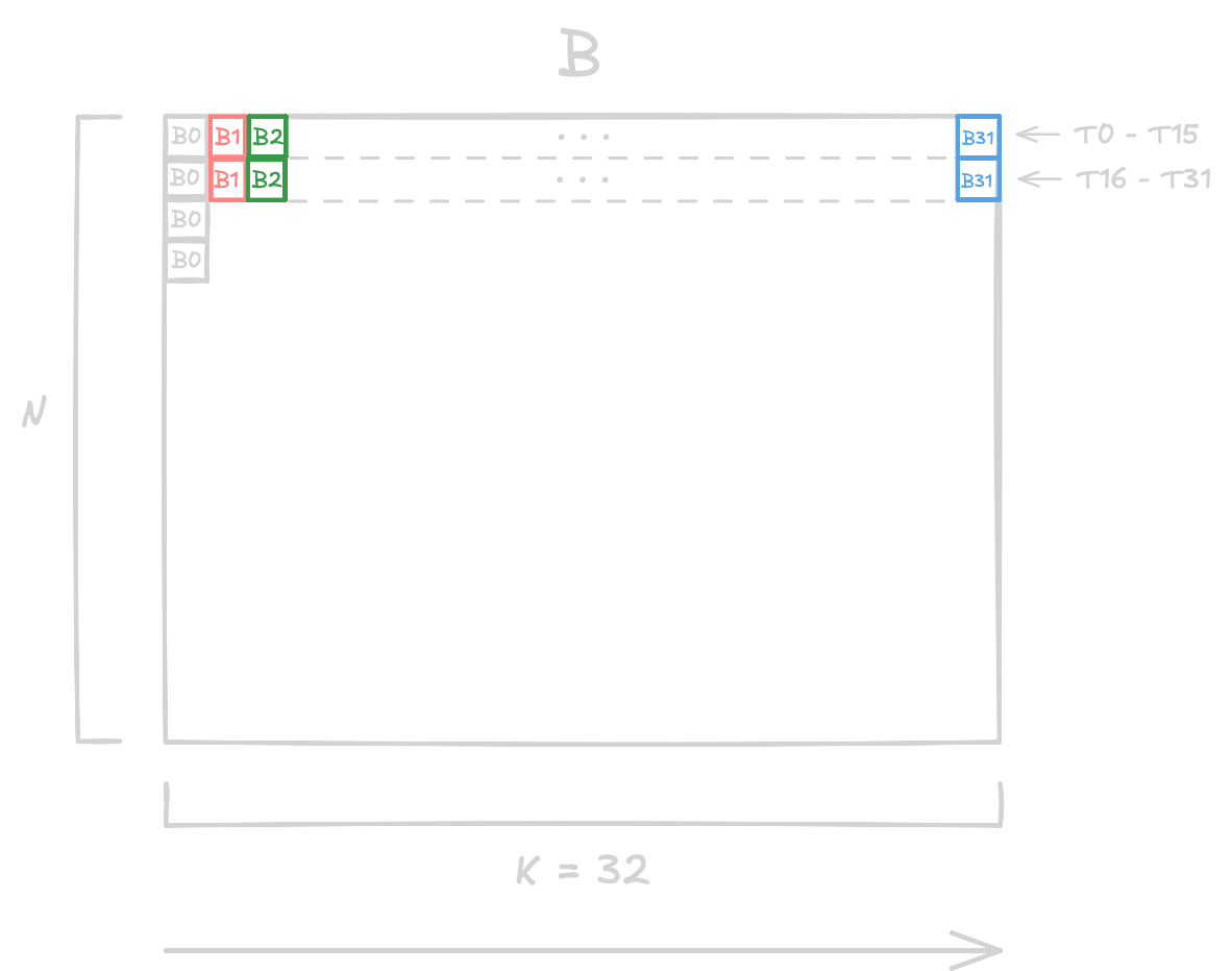
For each iteration across $K$, we observe that threads 0 through 15 will conflict with threads 16 through 31: a 2-way conflict.
Conflicts + Vectorized Instructions?
You may be wondering how bank conflicts occur when vectorized accesses come into play. For example, 128-bit reads/writes for each thread would span 4 banks simulatenously. Since all 32 banks can only service a maximum of 1024 bits per cycle, if every thread is making 128-bit reads for a total of 4096 bits across the warp, some lanes would need to request memory from the same bank by pigeonhole principle.
In this case, the banks split up the warp’s memory request into 4 phases, servicing 8 threads per phase, where phase 0 is threads 0-7, phase 1 is threads 8-15, and so on. Lanes in different phases may then access the same 4 banks and not considered be a conflict by ncu; lanes in the same phase need to stick to their respective banks.
Let’s talk solutions now. There are 2 common ways to solve conflicts:
- Padding - Pad SMEM with dummy memory to “push” data to certain banks. This is conceptually easier and straightforward to implement, but comes at the cost of wasting scarce SMEM.
- Swizzling - Re-map / swap certain blocks of SMEM addresses to control which data is under which bank. While a little harder to understand, swizzling adds very little overhead. We’ll look at this solution for our case.
An example swizzle for $B$ would be to swap the data in B0 and B1 in the second row. This way, data required for the first K-iteration can be serviced by both banks at once, rather than being serialized by one bank. We would repeat this pattern by swapping B2 with B3 for the second K-iteration, and so on. Typically, XOR is used in some way for remapping the SMEM addresses since it’s bijective (that is, $(x \oplus c) \oplus c = x$) and cheap. Recall its truth table:
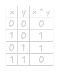
Applying this to the example, we can XOR addresses 32 and 33 with a fixed constant of 1, effectively swapping their addresses. Before this though, since we need to repeat this pattern every 2 rows for other warps, we first modulo the address by 64. To then leave the first of the 2 rows identity, we right-shift the modulo’d address by 5 (division by 32), and only then do we apply the XOR. All together: swizzled = addr ^ (addr % 64 >> 5).
We’ll now take a look at the slightly more complex CUTLASS API. For reference, the implementation is here . The docstring sheds some light:
// A generic Swizzle functor
/* 0bxxxxxxxxxxxxxxxYYYxxxxxxxZZZxxxx
 *                               ^--^ MBase is the number of least-sig bits to keep constant
 *                  ^-^       ^-^     BBits is the number of bits in the mask
 *                    ^---------^     SShift is the distance to shift the YYY mask
 *                                       (pos shifts YYY to the right, neg shifts YYY to the left)
 *
 * e.g. Given
 * 0bxxxxxxxxxxxxxxxxYYxxxxxxxxxZZxxx
 * the result is
 * 0bxxxxxxxxxxxxxxxxYYxxxxxxxxxAAxxx where AA = ZZ xor YY
 */
template <int BBits, int MBase, int SShift = BBits>
struct Swizzle { ... }Don’t worry if you don’t understand this at a first glance. What this API does is it effectively formalizes what we discussed in the previous example for more general power-of-2 swizzles in binary. I won’t delve into the implementation details (see the swizzling portion of Aleksa Gordic’s blog ), but rather what you as the user need to know to start using it.
The 3 parameters are used as follows: A bitmask of size BBits of 1s starting at bit SShift + MBase (zero-indexed) is bitwise ANDed with the input address. The resulting mask is then right- or left-shifted by SShift bits, depending on its sign, and XORed with the input address.
A couple things to note: The swizzle…
- acts as an identity function for any addresses below 2
SShift + MBase - operates at a “granularity” of
MBaseaddress indices. - must be applied to both the write and read side when using SMEM to ensure consistency.
- is applied as a composition on top of another layout, as we’ve seen earlier in the CuTe API.
Applying this to our example again, we need to check if the 5th bit of the input (corresponding to 32) is 1 by using a bitmask with a width of just 1 and shifting it down to the appropriate bit to XOR with. We know at this point that BBits = 1 and SShift + MBase = 5, since addresses below 32 should remain identity.
Now, you might be saying that MBase should be 0, since we XORed addresses by 1 earlier. This would be correct if we were solely considering the read side. However, recall that we used 128-bit copies in the GMEM → SMEM write side, which thus requires an alignment of 4 floats. Swizzling at a granularity of 1 address would break this alignment requirement. Instead, we need to swizzle at a minimum granularity of 4 address indices, meaning we should have MBase = 2 and SShift = 3. Finally, we have the new $B$ SMEM layout to be:
auto sB_layout_swizzled = composition(Swizzle<1,2,3>{}, sB_layout);

...

auto kernel = ampere_sgemm_128x32_3stage<decltype(stride_A), decltype(stride_B), decltype(stride_C),
                                         decltype(sA_layout),
                                         decltype(sB_layout_swizzled),
                                         decltype(cta_shape),
decltype(copy_A), decltype(copy_B), decltype(mma)>;No Modulo?
What ensures the swizzle pattern is identity for addresses 64-95, 128-159, and so on, but is still applied for addresses 96-127, 160-191, and so on? Note their binary representations. Since only the non-identity addresses would have a 1 in the 5th bit, we’re all set.
But suppose we did want a swizzle for these identity addresses. We would then widen the bitmask by increasing BBits to 2. Note that a restriction is that the bitmask must be of adjacent bits. But this is almost never a problem, since use-cases where non-adjacent bits are needed are rare (e.g. bitmask on bits 7 and 8 but XOR with bits 2 and 4).
wide epilogue instructions
This is not an optimization that was informed by profiling, but still worth chasing after. As mentioned earlier, the scattered register fragment per thread prevents us from using wide 128-bit global memory instructions. Recall that $C$ is column-major and has a stride of 1 along its M-mode. We should thus pack 4 values along the M-mode. Visualizing this change:

Changing the positions of $C$ that each thread computes requires a change in the thread-value mappings from TiledMMA. Thankfully, CuTe exposes a parameter in make_tiled_mma that lets us rearrange the mapping for situations like this.
// @tparam MMA_Atom The MMA_Atom to use in the TiledMMA
// @tparam AtomLayoutMNK The MNK-tiling of the Atom to be performed.
// @tparam PermuationsMNK Permutations to apply to each MNK-mode before tiling for the Atom.
template <class MMA_Atom,
          class AtomLayoutMNK,
          class PermutationMNK = Tile<Underscore,Underscore,Underscore>>
struct TiledMMA : MMA_Atom { ... }The two parameters following the MMA atom are…
AtomLayoutMNK, as the name suggests, lets us define the tiling of the “physical” hardware atom. We set the M- and N-mode tile sizes to 16 earlier, leaving the K-mode out since we don’t tile atoms across it.- Recall our $C$ tile size was 128 × 128, while our tiled physical atoms were 16 × 16.
TiledMMApartitioning automatically took care of logically replicating these atoms across the input tensor. This is related to why we launch the kernel withsize(mma)threads — with 16 × 16 = 256 physical atoms, we need precisely 256 threads.
- Recall our $C$ tile size was 128 × 128, while our tiled physical atoms were 16 × 16.
PermutationMNKlets us logically replicate the tiled atoms to a desired shape and apply a permutation on thread-value mappings along the MNK-modes.
In summary, these parameters control the arrangement of backing hardware atoms, the logical tiling of atoms to larger tensors, and the arrangement of values from these replicated tiles.
Let’s take a look at the code change:
auto mma = make_tiled_mma(
    MMA_Atom<UniversalFMA<float>>{},
    Layout<Shape<_16,_16>>{},
    Tile<
        Layout<Shape<_16,_4,_2>, Stride<_4,_1,_64>>,
        _128,
        _32
    >{}
);Taking a look at the 3rd argument, we see a Tile object, with three template args. corresponding to the MNK-modes respectively. The static integer arguments for the N- and K-modes indicate that we do not wish to apply a permutation to those modes. Instead, they represent identity functions. The actual values for N and K represent that we are logically extending the tiled MMA to the threadblock tile, which had $M = 128$, $N = 128$, and $K = 32$. Note that the size of the layout for the M-mode is also 128, but we are applying a permutation, so it’s not just an integer.
We can technically leave the N- and K-modes out since they’re just identity functions, and the tiled MMA will take care of logically extending to larger tiles on a partition without permutations, but we leave them here for clarity.
The layout for the M-mode can be read as a gather/scatter pattern. Given some an unpermuted M-mode index $x$, we apply the layout $f$ to get a new permuted index $y$. Recall that layouts are colexicographic, meaning that the left-most coordinate changes the “fastest”.
Examples
Suppose we wish to compute the new permuted index for values at $M_{\text{old}} = 2$. Going from the left, its hierarchical coordinate would then be $(2, 0, 0)$. Dotting this with the stride, we get that $M_{\text{new}} = 8$.
Consider values with $M_{\text{old}} = 33$. The left-most mode divides 33 twice, so the coordinate to its right should be 2, leaving a remainder of 1 in the left-most coordinate. All together, the coordinate would be $(1, 2, 0)$, which becomes $M_{\text{new}} = 6$.
CuTe’s crd2idx(Index, Shape) function can verify our results.
Looking at our layout: Layout<Shape<_16,_4,_2>, Stride<_4,_1,_64>>, it:
- Scatters contiguous groups of 16 values by 4 (e.g. 0 → 0, 1 → 4, …, 15 → 64)
- Gathers groups of 4 values strided by 16 to be contiguous (e.g. 16 → 1, 32 → 2, 48 → 3, …)
- Replicates this permutation twice strided by 64 to cover indices 64 through 127 (again, could be omitted since partition will take care of tiling the permuted pattern)
Great! Now, we need to tweak our epilogue to take advantage of the contiguous values. We allocate a temporary register buffer to hold 1 “column” of the 8 × 8 fragment at a time (could use more here), copy in the corresponding column from $C_{\text{in}}$ with 2× 128-bit instructions, apply axpby, and copy it out to $C_{\text{out}}$ with 2× 128-bit instructions.
auto tCgC_fragment = make_fragment_like(tCrC(_,_,0));  // (1,8) : (0,1)

for (uint col = 0; col < size<2>(tCgC); ++col) {
    copy(AutoVectorizingCopy{}, tCgC(_,_,col), tCgC_fragment);
    axpby(alpha, tCrC(_,_,col), beta, tCgC_fragment);
    copy(AutoVectorizingCopy{}, tCgC_fragment, tCgC(_,_,col));
}Lastly, note the use of AutoVectorizingCopy as the first argument. This allows copy to automatically dispatch to an instruction of the widest common alignment between the source and destination tensors.
conclusion
In this article, we’ve taken a deceivingly simple single-precision GEMM to a SOTA implementation on an older Ampere GPU, learning many CUTLASS CuTe concepts along the way. The more general techniques and optimizations we’ve touched on also apply to production kernels in deep learning libraries. The full code for this kernel is available here .
If you’ve made it this far, thank you for your attention; I really hope you were able to pick up a thing or two and gained an appreciation for how deep the kernel optimization rabbithole can get.